So, you want to know why we use mean moving range, mean(mR), and not standard deviation to determine XmR control limits. Before answering, let's do a quick review to make sure we are starting on the same page. The mean(mR) is determined by first finding the absolute difference between sequential pairwise measurements. This gives you a series of moving ranges – mR. Next, you calculate the mean of those ranges to give you mean(mR). Below are some sample calculations.
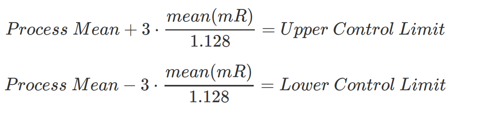
Once you've determined the mean(mR), you are in a position to calculate the sequential deviation: mean(mR) / 1.128. By multiplying the sequential deviation by ± 3, we can establish the XmR control limits around the mean. The process is summarized succinctly in the following expressions:
To learn more about the significance of constant 1.128 check out my article on XmR charting – control constant section.
Now that we are all on the same page. Why do we use mR to calculate XmR control limits? Why not just use 3 standard deviations around the mean and be done with it? This is a reasonable question. The answer is that the standard deviation, represents the total variation in our data. Total variation is comprised of random variation and systematic variation. When we make an XmR chart, our control limits should represent the random component to the variation in our process. We get this though the mR derived sequential deviation discussed above. The benefit of plotting the random variation window of our process (3 * sequential deviation), is that we can detect when systemic variation creeps into our process. And, hopefully do some corrective action to remove it.
So in short, mean(mR) gives us a sense of the random process variation and a way to detect systematic variation.
To help bring all this together, let's consider two extreme examples using a process for makeing 3 inch screws. The key process measure is length. Here are the deatils of the two cases:
Case 1: Screw lengths are statistically normal, identically distributed, and independent
Case 2: Screw lengths exhibit a systematic stepping pattern.
Case 1: Perfectly Normal Data
Suppose you sequentially sample 100, 3 inch screws from the process line. You measure them, and get the following lengths.
| ScrewID | 1 | 2 | 3 | 4 | 5 | 6 | 7 | 8 | 9 | 10 | 11 | 12 | 13 | 14 | 15 | 16 | 17 | 18 | 19 | 20 |
| Length | 2.92 | 2.96 | 2.86 | 3.04 | 3.07 | 2.85 | 3.00 | 2.92 | 2.97 | 2.97 | 3.09 | 3.07 | 2.99 | 3.06 | 3.05 | 3.02 | 3.07 | 2.91 | 3.07 | 3.20 |
| ScrewID | 21 | 22 | 23 | 24 | 25 | 26 | 27 | 28 | 29 | 30 | 31 | 32 | 33 | 34 | 35 | 36 | 37 | 38 | 39 | 40 |
| Length | 3.22 | 2.80 | 2.84 | 3.07 | 3.10 | 3.05 | 3.04 | 3.04 | 3.00 | 3.12 | 3.08 | 2.89 | 2.84 | 3.01 | 3.11 | 2.94 | 2.96 | 3.16 | 2.92 | 2.91 |
| ScrewID | 41 | 42 | 43 | 44 | 45 | 46 | 47 | 48 | 49 | 50 | 51 | 52 | 53 | 54 | 55 | 56 | 57 | 58 | 59 | 60 |
| Length | 3.06 | 2.94 | 3.02 | 2.88 | 3.03 | 2.89 | 3.06 | 3.09 | 3.11 | 3.04 | 2.95 | 2.95 | 3.21 | 3.11 | 3.09 | 2.94 | 3.09 | 2.98 | 3.18 | 3.01 |
| ScrewID | 61 | 62 | 63 | 64 | 65 | 66 | 67 | 68 | 69 | 70 | 71 | 72 | 73 | 74 | 75 | 76 | 77 | 78 | 79 | 80 |
| Length | 2.93 | 2.96 | 2.98 | 3.01 | 3.30 | 3.07 | 3.02 | 2.97 | 2.89 | 3.06 | 2.97 | 2.94 | 3.09 | 2.98 | 2.77 | 2.91 | 3.02 | 2.98 | 2.89 | 2.98 |
| ScrewID | 81 | 82 | 83 | 84 | 85 | 86 | 87 | 88 | 89 | 90 | 91 | 92 | 93 | 94 | 95 | 96 | 97 | 98 | 99 | 100 |
| Length | 3.15 | 3.12 | 3.20 | 3.15 | 3.04 | 2.98 | 3.07 | 3.03 | 3.01 | 2.99 | 3.06 | 3.13 | 3.03 | 3.20 | 2.85 | 3.14 | 2.98 | 3.11 | 3.00 | 3.08 |
You prepare to make your XmR chart, and calculate the following items:
- mean: 3.0186
- mean(mR): 0.1054545
- sequential deviation: 0.0934881
- standard deviation: 0.0989135
Comparing the results for sequential deviation and the standard deviation, you conclude that there was very little point in determining the mean(mR). In this case, you would be correct. But, watch what happens when the data is not perfect, suppose it has systematic variations as in the second case described below.
Case 2: Systematic Variations
Some time passes and again you sequentially sample 100, 3 inch screws from the process line. You measure them, and get a new set of lengths listed here.
| ScrewID | 1 | 2 | 3 | 4 | 5 | 6 | 7 | 8 | 9 | 10 | 11 | 12 | 13 | 14 | 15 | 16 | 17 | 18 | 19 | 20 |
| Length | 3.11 | 3.37 | 3.16 | 3.04 | 3.13 | 3.13 | 3.25 | 3.28 | 3.15 | 3.21 | 3.22 | 3.09 | 3.10 | 3.30 | 3.23 | 3.26 | 3.41 | 3.36 | 3.26 | 3.22 |
| ScrewID | 21 | 22 | 23 | 24 | 25 | 26 | 27 | 28 | 29 | 30 | 31 | 32 | 33 | 34 | 35 | 36 | 37 | 38 | 39 | 40 |
| Length | 3.03 | 2.86 | 2.88 | 2.63 | 2.84 | 2.87 | 2.85 | 2.83 | 2.83 | 2.85 | 2.79 | 2.77 | 2.84 | 2.69 | 2.79 | 2.93 | 2.68 | 2.99 | 2.78 | 2.91 |
| ScrewID | 41 | 42 | 43 | 44 | 45 | 46 | 47 | 48 | 49 | 50 | 51 | 52 | 53 | 54 | 55 | 56 | 57 | 58 | 59 | 60 |
| Length | 3.22 | 3.00 | 3.07 | 2.94 | 2.89 | 3.11 | 3.06 | 2.92 | 2.94 | 2.95 | 2.79 | 3.01 | 2.93 | 3.10 | 3.08 | 3.07 | 2.99 | 3.03 | 3.05 | 2.93 |
| ScrewID | 61 | 62 | 63 | 64 | 65 | 66 | 67 | 68 | 69 | 70 | 71 | 72 | 73 | 74 | 75 | 76 | 77 | 78 | 79 | 80 |
| Length | 2.53 | 2.47 | 2.64 | 2.46 | 2.66 | 2.68 | 2.69 | 2.62 | 2.60 | 2.50 | 2.74 | 2.40 | 2.69 | 2.56 | 2.56 | 2.67 | 2.55 | 2.72 | 2.63 | 2.70 |
| ScrewID | 81 | 82 | 83 | 84 | 85 | 86 | 87 | 88 | 89 | 90 | 91 | 92 | 93 | 94 | 95 | 96 | 97 | 98 | 99 | 100 |
| Length | 3.23 | 3.27 | 3.36 | 3.29 | 3.26 | 3.20 | 3.24 | 3.22 | 3.13 | 3.17 | 3.28 | 3.17 | 3.12 | 3.26 | 3.31 | 2.98 | 3.24 | 3.19 | 3.28 | 3.10 |
You prepare to make your chart. Like before, you calculate the following items:
- mean: 2.9737
- mean(mR): 0.1160606
- sequential deviation: 0.1028906
- standard deviation: 0.2531565
Interestingly, we have the same mean but the standard deviation value is more than 2X the sequential deviation. Let's compare results from case 1 and case 2 side by side to see what else we can learn.
| Case 1 (Perfect Process) | Case 2 (Stepped) | |
|---|---|---|
| mean | 3.02 | 2.97 |
| sequential deviation | 0.093 | 0.103 |
| standard deviation (sd) | 0.099 | 0.253 |
Comparing the cases, we see that the mean value is ~3 inches in both. Values for sequential deviation and standard deviation look similar in case 1, but they are very different in case 2. Sequential deviations derived from mean(mR) are strikingly similar for the two case. Finally, we note that the standard deviations between the two cases are strikingly different. This is a demonstration that the mean(mR) and derived sequential deviation are less sensitive to the systematic variations.
Effect on XmR Control Limits
Let's look at the control charts, to see if there is anything interesting to see. When you make the plots, you use red lines for the mR calculated limits and green lines for the standard deviation based XmR control limits.
In the plot with the perfect data, the green standard deviation and red mR based limits are very similar. If you had millions of data points there would in fact be no difference to observe. This is after all how we simulated the value of the XmR control constant 1.128. Now, the stepped data is much more interesting. Look how much wider the green standard deviation based limits are vs those in the perfect data. Also notice that the mean and mR based limits for both cases are essentially the same. The difference you are seeing between the green standard deviation limits and the red mR limits in the stepped example is because
- the standard deviation based XmR control limits are influenced strongly by systematic variation. This inflates our limits, making it difficult to detect assignable cause variations.
- The mR based limits, suppress (not eliminate) the influence of systematic variation. Because of this suppression, our XmR control limits more accurately reflect our random process variation. This allows for better detection of assignable cause variations.
To illustrate this, let's look at the sample plots with their mR data included. For now don't worry about the red control limit lines around the mR data.
The mR data for Case 1 and 2 is similarly centered and distributed, despite the systematic offsets in case 2. The result is very similar values for mean(mR) and ultimately similar values for sequential deviation in both cases. If the systematic offsets in the stepped case were bigger, we would see more pronounced spikes in the mR data. Such spikes could inflate the mean(mR) value and our XmR control limits. However, the inflation will be much less than that observed with standard deviation based limits (green lines).
Summary
When preparing an XmR chart, we use the mean moving range, mean(mR), to determine the sequential deviation and the control limits. XmR control limits base on mean(mR) are less biased by systematic process offsets. As a result, mR based control limits:
- give a clearer view of random error in our processes.
- allow us to calculated XmR control limits that can detect systematic(assignable cause) variation, which we are trying to eliminate.
2 Comments
Pingback:
Pingback: